PNA Quality Control
This tutorial details the first steps of data analysis to quality control and clean up the PNA data output from Pixelator.
After completing this tutorial, you should be able to:
- Use the molecule rank plot to manually set cell calling thresholds and filter out low-quality cells.
- Visualize sample-level QC metrics such as the number of cells.
- Check distributions of quality metrics, protein counts (molecules) and read depth.
- Identify and remove cell outliers using the antibody count distribution metric Tau.
Setup
First, we will load packages necessary for downstream processing.
library(pixelatorR)
library(dplyr)
library(stringr)
library(SeuratObject)
library(here)
library(ggplot2)
library(tidyr)
library(tibble)
Load data
We will begin by loading the merged dataset we created the end of the previous tutorial Data handling. As described previously, this merged object contains two samples: one with resting PBMCs and one with PHA-stimulated PBMCs. Note that if you continue directly from the previous tutorial, you don’t need to load the data again.
DATA_DIR <- "path/to/local/folder"
Sys.setenv("DATA_DIR" = DATA_DIR)
# Load the object that you saved in the previous tutorial. This is not needed if it is still in your workspace.
pg_data_combined <- readRDS(file.path(DATA_DIR, "combined_data.rds"))
pg_data_combined
An object of class Seurat
158 features across 2137 samples within 1 assay
Active assay: PNA (158 features, 158 variable features)
 1 layer present: counts
Cell calling: Molecule rank plot
Here, we use the molecule rank plot to perform a more fine-tuned quality control of the called cells and make a manual adjustment to the number of cells that were called by Pixelator if needed. Pixelator automatically determines a threshold to exclude small components and if this threshold is lower than 8000 molecules, Pixelator will adjust the threshold to 8000. If you expect to find small cells in your sample, such as platelets, you might want to adjust this threshold in Pixelator to a lower value.
Here, the goal is to remove small components which might not represent whole cells.
# Plot the molecule rank plot
molecule_rank_plot <- MoleculeRankPlot(pg_data_combined, group_by = "condition")
molecule_rank_plot
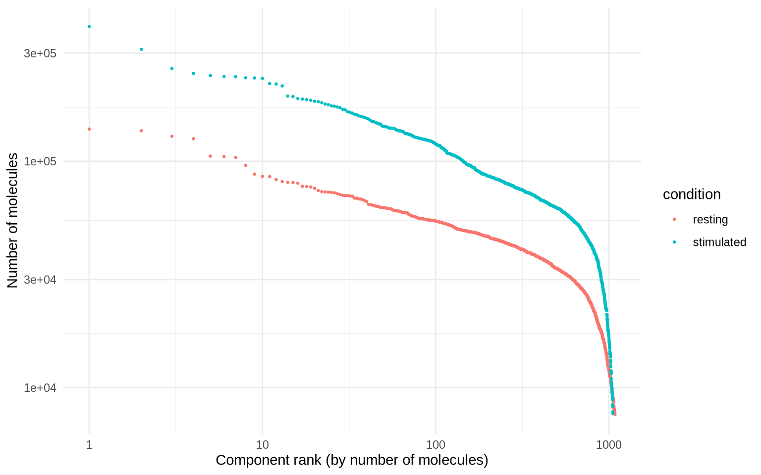
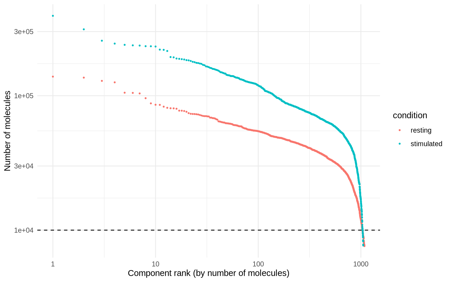
It looks like components are declining rapidly in size at around 10000 UMIs, so we will set a manual cutoff at that point, represented by a dashed line in the plot below.
cutoff <- 10000
molecule_rank_plot +
  geom_hline(yintercept = cutoff, linetype = "dashed")
# Filter cells to have at least 10000 molecules
pg_data_combined <- pg_data_combined %>%
  subset(n_umi >= cutoff)

pg_data_combined
An object of class Seurat
158 features across 2074 samples within 1 assay
Active assay: PNA (158 features, 158 variable features)
 1 layer present: counts
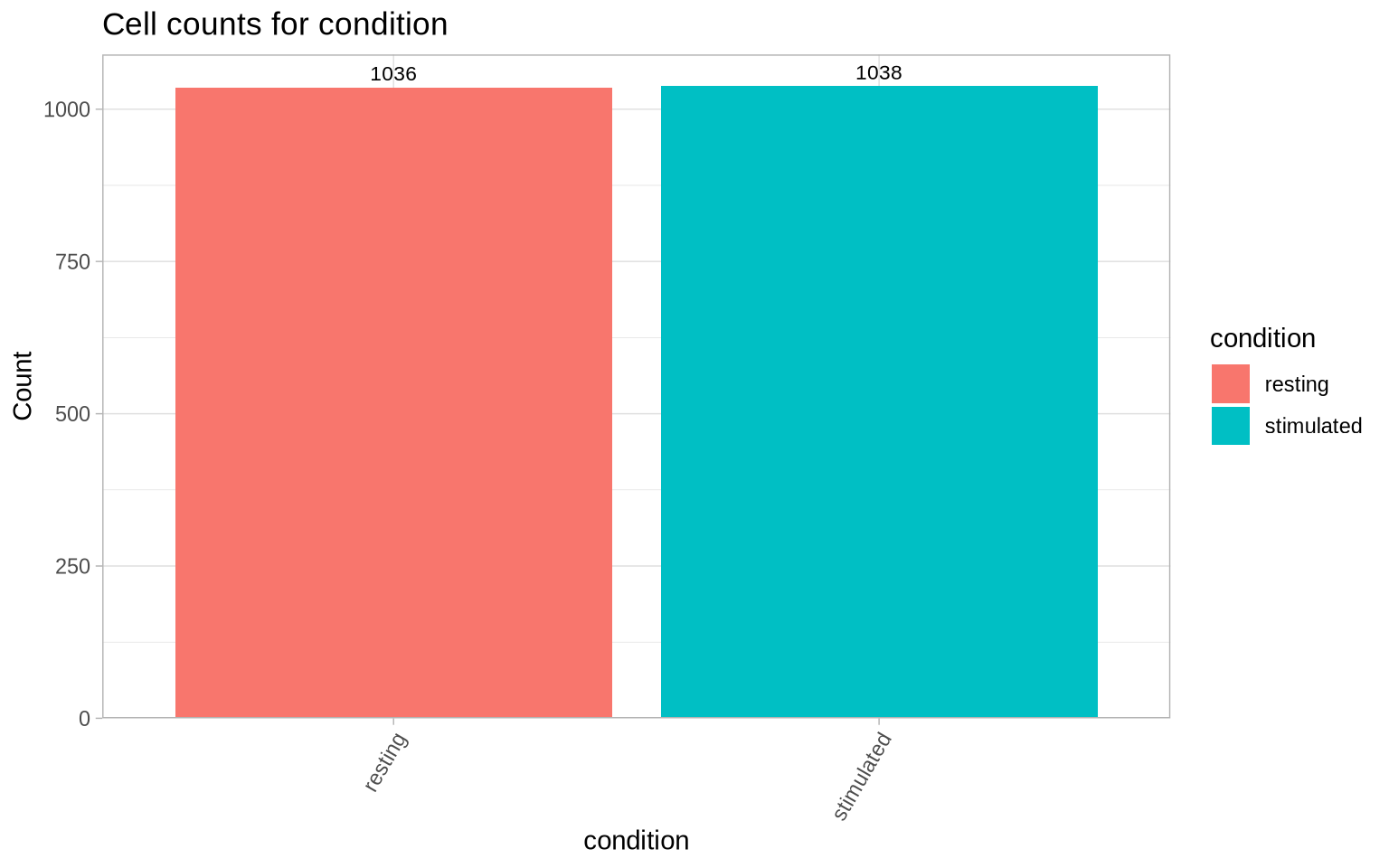
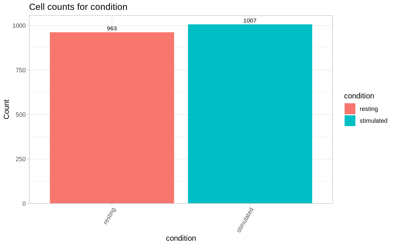
Now we can inspect the number of called cells per condition after filtering out small cells. The observed numbers of cells are close to the expectation of 1000 cells per condition.
CellCountPlot(pg_data_combined, color_by = "condition")
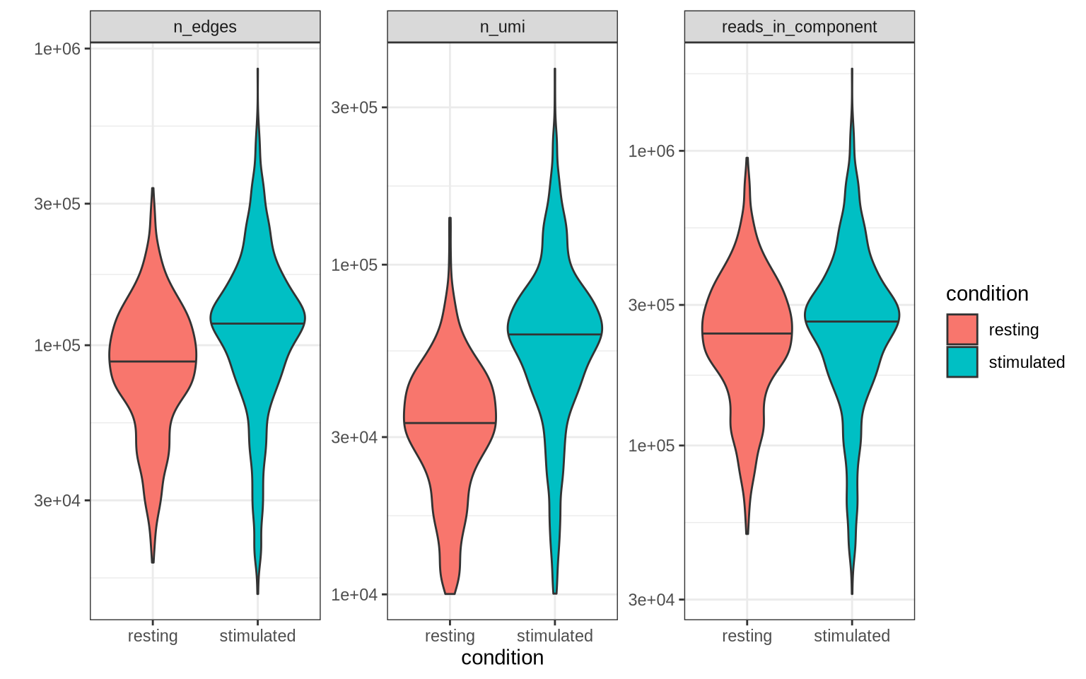
Other QC metrics can also be useful to explore. In the plot below we
check the distribution of number of protein molecules (n_umi), number
of edges (n_edges) and number of reads per component
(reads_in_component) across the two conditions.
pg_data_combined[[]] %>%
  select(condition, n_umi, reads_in_component, n_edges) %>%
  pivot_longer(cols = c("n_umi", "n_edges", "reads_in_component"), names_to = "metric", values_to = "value") %>%
  ggplot(aes(condition, value, fill = condition)) +
  geom_violin(draw_quantiles = 0.5) +
  facet_wrap(~ metric, scales = "free_y") +
  scale_y_log10() +
  theme_bw() +
  labs(y = "")
Antibody count distribution outlier removal
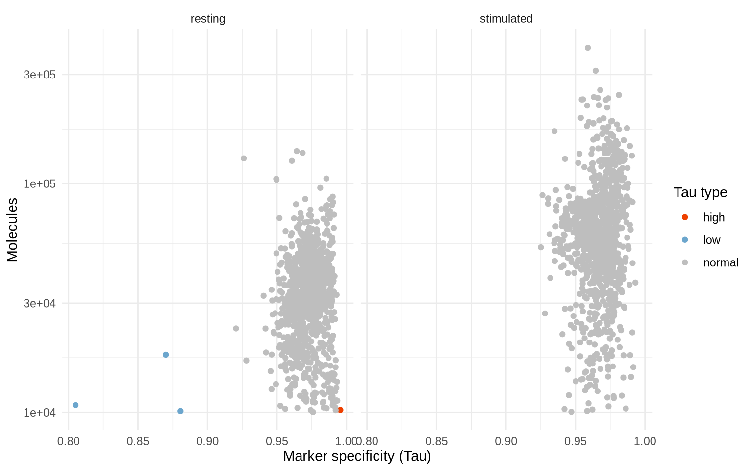
Below, we have plotted the number of molecules against Tau, and colored each cell by Pixelator’s classification of Tau (low, normal, or high). In short, Tau measures the heterogeneity of protein composition which can be used to detect various types of outliers. Here we see some cells with a low Tau score that might be antibody aggregates. Cells with high Tau have low specificity and could for instance include a more heterogeneous composition of proteins than we would expect from a normal cell. As these outliers likely represent technical artefacts, we will remove them from the dataset.
# Custom plot to visualize the Tau distribution
TauPlot(pg_data_combined, group_by = "condition")
# Only keep the components where tau_type is normal
pg_data_combined <- pg_data_combined %>%
    subset(tau_type == "normal")

pg_data_combined
An object of class Seurat
158 features across 2070 samples within 1 assay
Active assay: PNA (158 features, 158 variable features)
 1 layer present: counts
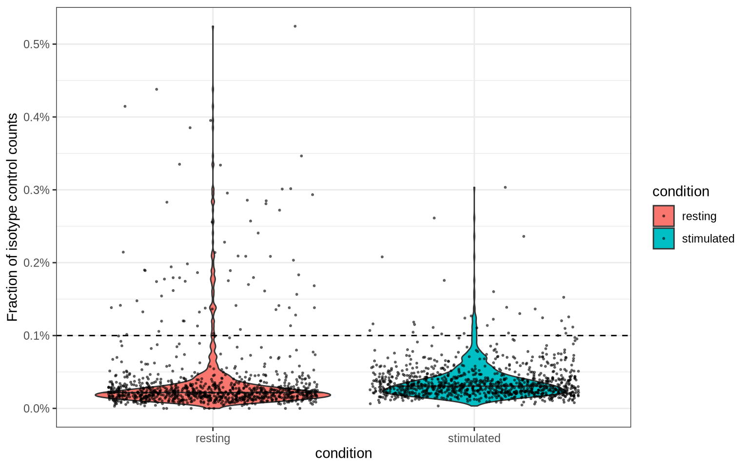
Isotype control levels
PNA data includes three isotype control antibodies which are used to measure the background signal (non-specific binding). The abundance levels for these isotype controls should be low in comparison to the other antibodies. Elevated levels can therefore be used to identify low-quality cells that should be removed.
Based on the distribution of the isotype control levels plotted below, a cutoff at 0.1% seems to get rid of a handful of outliers.
isotype_controls = c("mIgG1", "mIgG2a", "mIgG2b")

isotype_control_fraction_cutoff <- 0.001

pg_data_combined[[]] %>%
  select(condition, isotype_fraction) %>%
  ggplot(aes(condition, isotype_fraction, fill = condition)) +
  geom_violin(draw_quantiles = 0.5) +
  geom_jitter(size = 0.4, alpha = 0.5) +
  theme_bw() +
  labs(y = "Fraction of isotype control counts") +
  scale_y_continuous(labels = scales::percent) +
  geom_hline(yintercept = isotype_control_fraction_cutoff, linetype = "dashed")
Now let’s apply this cutoff to remove cells with elevated isotype control levels from our dataset:
pg_data_combined <- pg_data_combined %>%
    subset(isotype_fraction < isotype_control_fraction_cutoff)

pg_data_combined
An object of class Seurat
158 features across 1970 samples within 1 assay
Active assay: PNA (158 features, 158 variable features)
 1 layer present: counts
Let’s check again how many cells we have left after filtering:
CellCountPlot(pg_data_combined, color_by = "condition")
Going through the above steps we have performed a basic quality control to filter out small cells, Tau outliers and cells with elevated isotype control levels. These filters take us quite far in the QC process, and we encourage users to adjust metric filtering thresholds based on the metric distributions. Depending on the sample type, it can be a good idea to explore other metrics as well. With a clean, high-quality PNA dataset in hand, we are ready to proceed to the next step, in which we will be normalizing and denoising protein abundance data to facilitate cell type annotation.
If you want to pause here and save the filtered data for the next tutorial, you can do so with the following code.
# Save filtered dataset for next step. This is an optional pause step; if you prefer to continue to the next tutorial without saving the object explicitly, that will also work.
saveRDS(pg_data_combined, file.path(DATA_DIR, "combined_data_filtered.rds"))