Data Integration
This tutorial demonstrates how to integrate multiple single-cell omics datasets in R using the Harmony method. Harmony is a popular data integration technique, and for a broader overview of available methods, you can consult this benchmark paper.
We will guide you through the steps of data preprocessing, dimensionality reduction, dataset harmonization using Harmony, and visualization of the integrated results.
After completing this tutorial, you should be able to:
- Preprocess single-cell data: normalize, scale, and identify variable features.
- Perform dimensionality reduction using PCA and UMAP, and visualize the resulting embeddings.
- Integrate multiple datasets using the Harmony method.
- Evaluate the success of data integration through visualization.
Setup
library(pixelatorR)
library(dplyr)
library(tibble)
library(stringr)
library(tidyr)
library(Seurat)
library(ggplot2)
library(here)
library(harmony)
library(pheatmap)
Load data
To illustrate the integration procedure we continue with the normalized object we created in the previous tutorial. As described before, this merged object contains two samples: a resting and PHA stimulated PBMC sample.
DATA_DIR <- "path/to/local/folder"
Sys.setenv("DATA_DIR" = DATA_DIR)
# Load the object that you saved in the previous tutorial. This is not needed if it is still in your workspace.
pg_data_combined <- readRDS(file.path(DATA_DIR, "combined_data_normalized.rds"))
pg_data_combined
An object of class Seurat
158 features across 1970 samples within 1 assay
Active assay: PNA (158 features, 158 variable features)
 3 layers present: counts, data, scale.data
 2 dimensional reductions calculated: pca, umap
Harmonizing data
Data integration is frequently employed to address variability arising from technical or biological factors such as collection site, batch, experimental conditions, or time points. The goal of integration is to identify corresponding cell populations across different samples, enabling meaningful comparisons under varying conditions.
Data integration should be applied strategically to address specific biases impacting analysis. In this study, we are comparing samples subjected to distinct treatments (PHA stimulated vs. resting). Therefore, integration may be necessary to account for differences between the two conditions, facilitating more accurate comparisons and cell type annotation. Our aim is to identify shared cell populations across samples and conditions, ensuring we are comparing equivalent cell types.
To begin the integration process, we first need to assess whether a significant bias exists in our data. Let’s examine the UMAP visualization we recently generated to identify any clear separation between samples.
DimPlot(pg_data_combined, reduction = "umap", group.by = "condition") +
  coord_fixed()
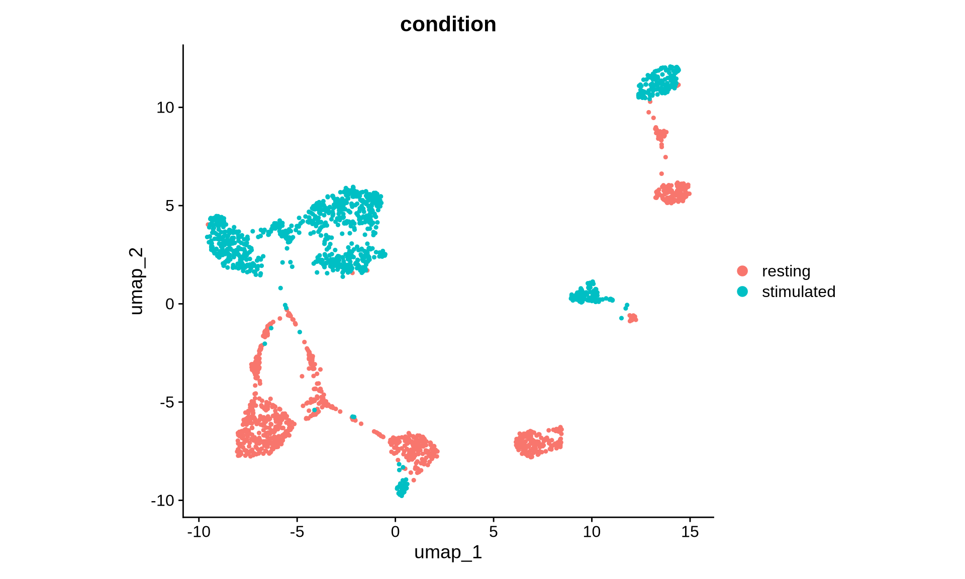
As suspected, the UMAP visualization reveals a clear separation of cells based on experimental condition, suggesting significant differences in protein abundance. To confirm that major immune cell types are present across all samples and conditions, let’s examine the abundance of specific marker proteins.
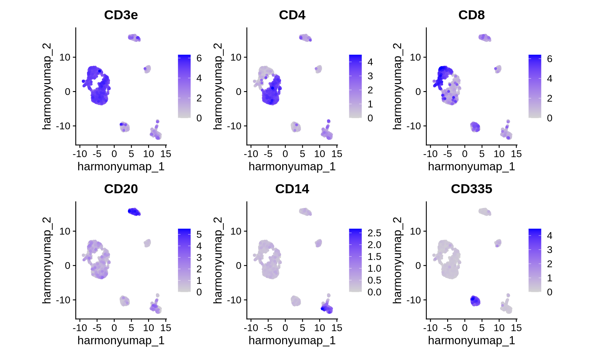
FeaturePlot(pg_data_combined,
            features = c("CD3e", "CD4", "CD8", "CD20", "CD14", "CD335"),
            reduction = "umap", ncol = 3,
            min.cutoff = 0,
            order = TRUE,
            coord.fixed = TRUE)
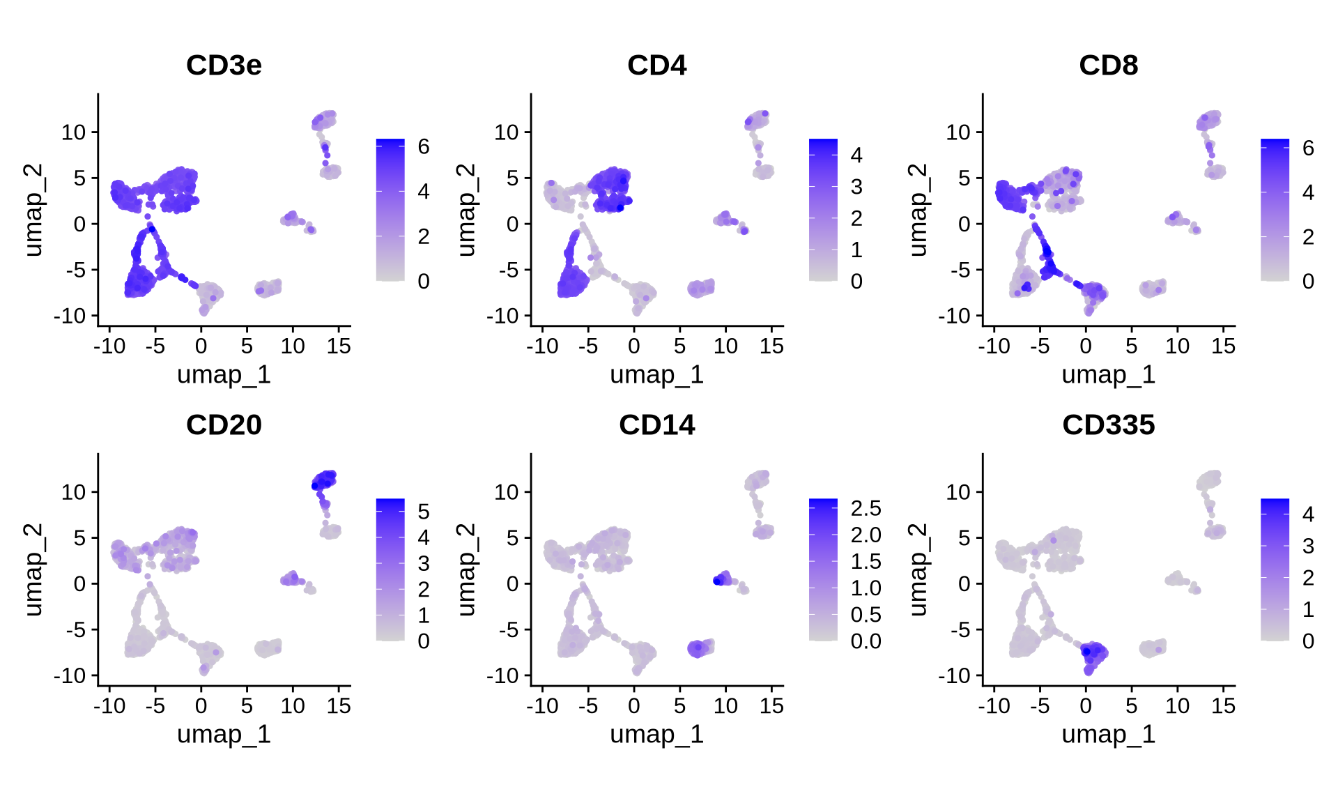
Examination of these markers confirms the presence of T helper cells (CD3+, CD4+), cytotoxic T cells (CD3+, CD8+), B cells (CD20+), monocytes (CD36+), and NK cells (CD335+) in both conditions. However, the distinct separation of these cell types by condition in the UMAP space indicates variations in protein abundance.
Clustering the non-integrated data could lead to condition-specific clusters for each cell type, hindering comparisons of protein abundance and spatial scores across samples. To address this, we will use the Harmony method to integrate the data and correct for sample- and condition-specific biases.
Our goal is to compare protein abundance in corresponding cell types
across different conditions. Therefore, we need a correction method that
preserves these biological differences while enabling meaningful
comparisons. Harmony achieves this by adjusting the existing PCA
embedding based on specified covariates, in our case the condition
variable. Harmony generates a new embedding, which we will use in place
of PCA for downstream analyses like UMAP and clustering. We previously
added the condition metadata to the Seurat object using AddMetaData to
facilitate this correction.
# Run Harmony to correct for donor effects
pg_data_combined <- pg_data_combined %>%
RunHarmony(group.by.vars = "condition",
reduction = "pca",
reduction.save = "harmony")
# Run UMAP on the Harmony embedding
pg_data_combined <- pg_data_combined %>%
RunUMAP(reduction = "harmony", dims = 1:10,
reduction.name = "harmony_umap")
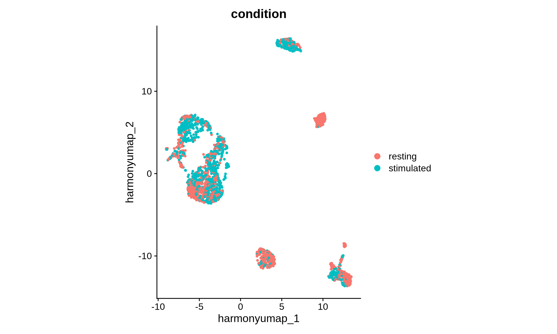
DimPlot(pg_data_combined, reduction = "harmony_umap", group.by = "condition", shuffle = TRUE) +
coord_fixed()
DimPlot(pg_data_combined,
  reduction = "harmony_umap",
  group.by = "condition",
  split.by = "condition")
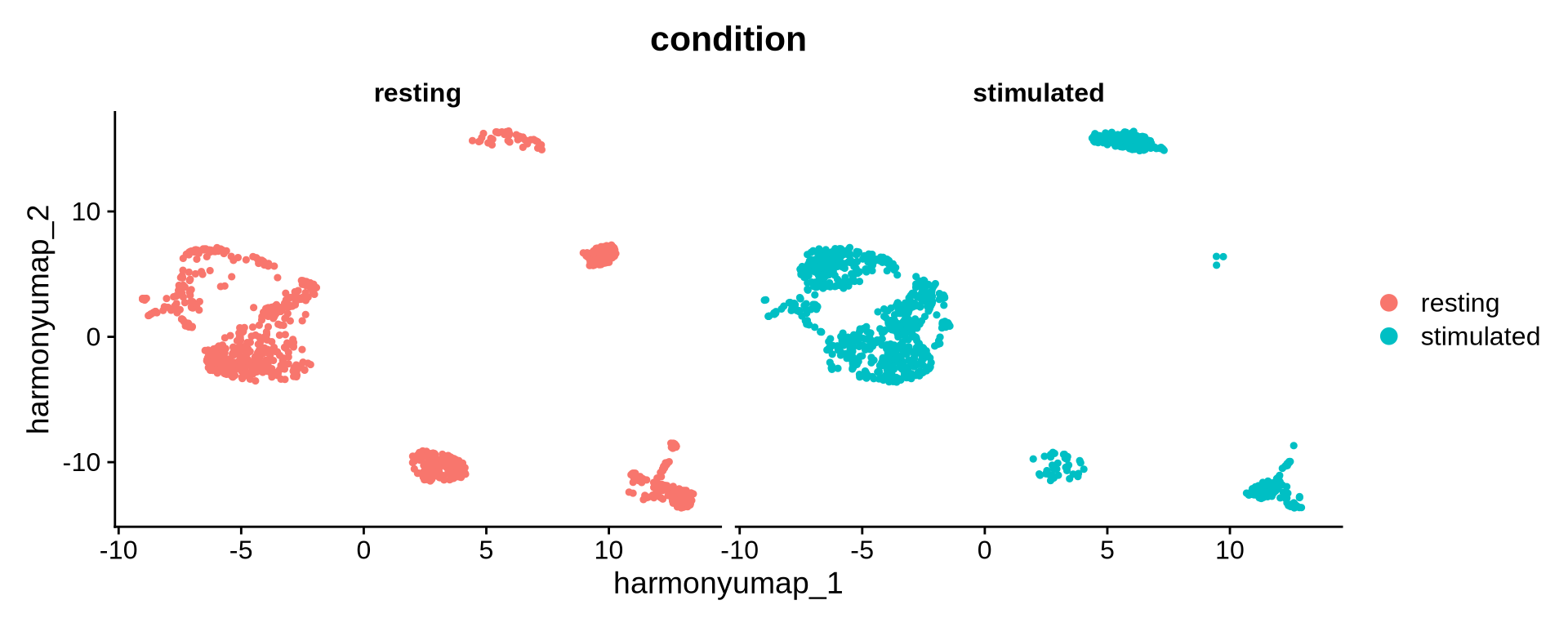
The UMAP visualization based on the Harmony embedding now shows greater overlap between samples. We observe clusters shared across conditions as well as some that appear condition-specific. Let’s now compare this Harmony-derived UMAP with the one generated from the original PCA embedding.
FeaturePlot(pg_data_combined,
            features = c("CD3e", "CD4", "CD8", "CD20", "CD14", "CD335"),
            reduction = "harmony_umap", ncol = 3,
            min.cutoff = 0,
            order = TRUE,
            coord.fixed = TRUE)
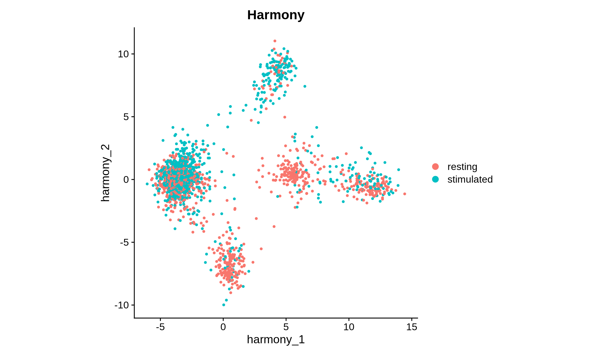
We can also visualize selected vectors from the PCA and harmony embeddings, showcasing that harmony has effectively aligned these across the two conditions.
DimPlot(pg_data_combined, reduction = "pca", group.by = "condition", shuffle = TRUE) +
  ggtitle("PCA") +
  coord_fixed()
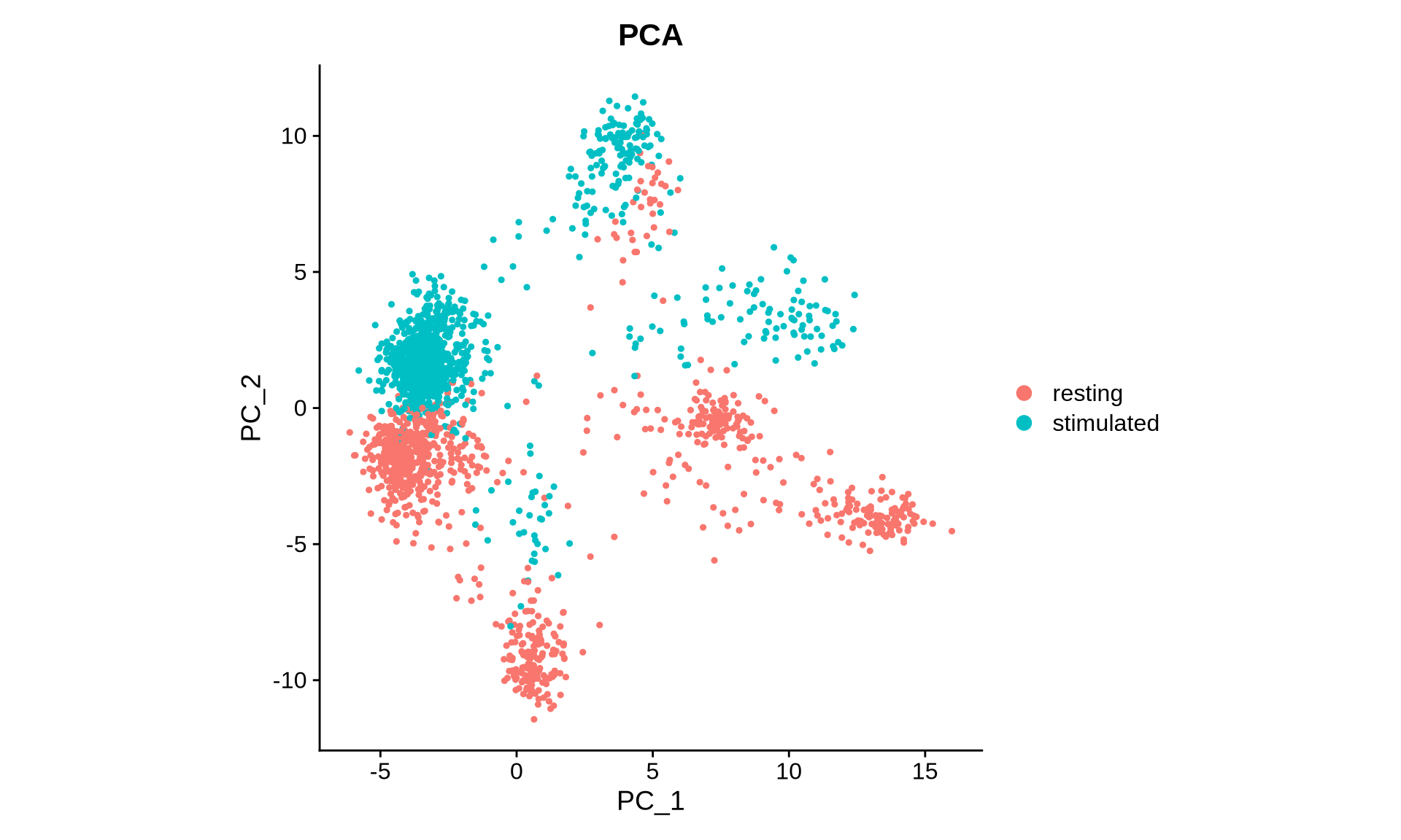
DimPlot(pg_data_combined, reduction = "harmony", group.by = "condition", shuffle = TRUE) +
  ggtitle("Harmony") +
  coord_fixed()
Let’s save this integrated object now for the next tutorial on Cell Annotation.
# Save filtered dataset for next step. This is an optional pause step; if you prefer to continue to the next tutorial without saving the object explicitly, that will also work.
saveRDS(pg_data_combined, file.path(DATA_DIR, "combined_data_integrated.rds"))
In this tutorial, we demonstrated how to integrate multiple PNA datasets using the Harmony method and perform downstream analysis on the integrated data. This approach is valuable for comparing samples from different donors, conditions, or time points when biological or technical variations in protein abundance could confound clustering and cell annotation. By applying Harmony, we can effectively correct for such factors, enabling meaningful cross-sample comparisons.