Algorithms
This section aims to explain briefly some of the algorithms used in pixelator. For extended explanations, if relevant, we try to include references in each sub-section.
Edge Collapsing
From the sampled NGS reads, pixelator tries to reconstruct the original molecules that have been assayed by MPX. In order to achieve this, we use the combination of the antibody barcode, the UMI and UPIA to uniquely associate all UPIBs that show that fragment combination in the reads. Once that is done, after translating each nucleotide sequence to a binary sequence (using 2-bit encoding), we use Annoy (Approximate Nearest Neighbors Oh Yeah) to cluster those fragments at a certain Hamming distance from each other (default: 2 mismatches). The algorithm will then group a set of Ab/UMI/UPIA fragments into different groups where all fragments are separated just by less than the given Hamming distance from each other.
The reason to use Annoy is that many to many comparisons takes a lot of time. Performance in a worst case scenario is O(N^2) algorithm. On the other hand, Annoy is very quick and reduces the time complexity to O(log N).
Along the groups of fragments, pixelator creates a frequency table and we pick the most frequent UPIB and associate that with the Ab/UMI/UPIA fragment. That fragment combination with most frequent UPIB becomes the representative molecule or edge from each of the groups. Pixelator stores all edges in a large table, and for each edge it computes the total count of UPIBs (associated to the number of reads of a certain molecule), the number of fragments, and the total number of unique UPIBs.
The number of resulting edges is dependant on many factors: the origin of the cells, the experimental conditions (e.g. any stimulation of the cells), the number or reads sequenced for the library, and the number of cells in the experiment.
Multiplet recovery
From the edge list, pixelator generates an undirected bipartite graph where each Ab/UMI combination forms an edge, and each UPIA and UPIB form a node. Each graph is a representation of a putative cell but at this stage of the pipeline we use the concept of a component to refer to them.
![]()
Due to the complex nature of the assay biochemistry and the fact that the reaction is carried on a
single tube, MPX edge lists may have a proportion of undesired artefactual edges. Those few edges (
only a small proportion of the total edge number of the experiment) are removed in a step we call *
multiplet recovery* in the graph pipeline stage if the --multiplet-recovery removal flag is
activated (by default it is on).
This removal is achieved by using community detection algorithms that operate on the graph. Densely connected communities are assumed to represent cells and pixelator removes any spurious edges connecting them. Each component of the resulting edge list is assigned a recovered ID and pixelator saves a table of all the recovered IDs in relation to original IDs.
Edge Rank Plot and Cell Calling
The edge rank plot is a useful tool to visualize the range and distribution of antibody counts ( edges) across cells called by pixelator, and to help you to assess the data quality. The edge rank plot is constructed by visualizing all graph components (cells) ranked from highest to lowest by the number of unique antibodies (edges). * Pixelator* uses the edge rank plot internally to perform an automatic cell calling by finding the threshold point which distinguishes real cells from a background of small spurious components. The threshold is recognized as the elbow point, where the component size (edges) rapidly declines in relation to the rank. Although this process is automatic, it is advisable to plot the edge rank plot and set a manual cutoff to refine the selection of cells. The cutoff should be selected to approximate the elbow point where the component size is sharply declining in relation to the size rank. The number of edges that corresponds to an appropriate cutoff will vary depending on the dataset, as the number of molecules detected varies by multiple factors, such as sequencing depth, cell type, cell size, and cell states, such as whether the cell has undergone any type of stimulation or not.
![]()
Antibody Count Distribution Outliers
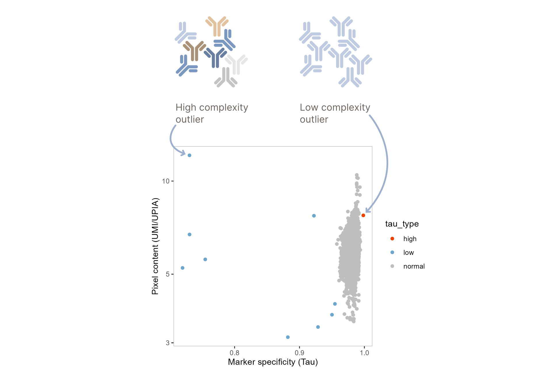
Cell components might rarely have a diverging distribution of counts across proteins, such that the
counts might be skewed to a single
protein or evenly distributed to most proteins. This can be an indication that the component is not
originating from
a cell, and could instead originate from debris or from an antibody aggregate. Antibody aggregates
form rarely,
and usually have either high complexity, consisting of wide range of different antibodies, or low
complexity, mainly constituted
by a single antibody. Pixelator detects these by using the metric Tau (tau), adjusted
from Yanai et al.,
which measures the skewness of antibody counts across different antibodies for a given component.
Tau is a numerical value
ranging from 0 and 1 describing the degree to which skewness the distribution of counts across
markers. A Tau of 0 indicates
equal distribution of counts across all antibodies and a Tau of 1 indicates that all counts are
distributed to a single antibody.
Pixelator classifies components by their Tau score in tau_type as high if the Tau score is
above 0.995 or deviates from the
population median with more than 2 interquartile ranges (IQRs), and as low if the Tau score is
lower than 5 IQRs from the
population median. If the tau_type is neither high or low, the tau_type is set to normal.
A typical down-stream
quality control will involve removing components marked as high or low tau_type.
Additionally, aggregates often have dense pixels with higher levels of antibodies detected per each
pixel, which can be measured
using the mean_umi_per_upia metric stored in the component meta data.
Spatial scores
Spatial structure can be challenging to describe in simple terms, particularly when assessing these structures across thousands of cells and numerous proteins.
In MPX and PNA data, spatial scores are used to analyze spatial relationships between proteins in cells. These scores are helpful to understand global spatial patterns within a cell or among cell populations and can be used to measure differences between cell populations or samples. The score simply measures spatial patterns by comparing observed spatial patterns against what would occur by random chance.
PNA Proximity Scores
The Proximity scores quantify the spatial correlation between pairs of proteins, allowing us to hypothesize about
spatial patterns on the cell surface, such as protein polarization, clustering, and protein complex formation.
To understand these scores, it’s helpful to first consider how a cell is represented in a Protein Network Assay (PNA)
data set.
In a Protein Network Assay data set, a cell is represented as a graph, where each node represents a single protein,
and the edges between nodes indicate spatial proximity—i.e., proteins that are located close to one another on the cell
surface.
Spatial correlation between pairs of proteins is measured by counting the edges connecting them, yielding a number
called the join count. If the join count for a protein pair is
high, it could indicate that these proteins are spatially correlated on the cell surface. However, we cannot
immediately draw this conclusion, because the join count is influenced by the abundance of the two proteins.
For instance, if both proteins are highly abundant, there is a higher chance of observing many edges between them
(a high join count) simply due to their greater availability.
To account for this, the Proximity scores compare the observed join count to the expected join count
(join_count_expected_mean) under random conditions, accounting for their relative abundances.
This adjustment aims to make the score reflect true spatial correlation rather than random chance.
The expected join count is estimated using random permutations. In each permutation, protein labels (node identifiers)
are shuffled while preserving the graph structure, including edge placement. For each shuffled graph, the join count
between protein pairs is recalculated. Repeating this process generates a distribution of join counts under random
conditions. From this distribution, we calculate the join_count_expected_mean (the average expected join count)
and the join_count_expected_sd (the standard deviation of these counts). These values provide a baseline for
determining whether the observed join count deviates significantly from random expectation.
With these three values—the observed join_count, the join_count_expected_mean, and the
join_count_expected_sd — we can compute the Proximity scores.
The first score is a Z-score, which measures how far the observed edge count is from the expected value,
measured in standard deviations. The formula for the Z score is:
Where:
x is the observed join_count (the actual number of edges)
μ is the join_count_expected_mean (the average number of edges from the permutations)
σ is the join_count_expected_sd (the standard deviation of the permuted edge counts)
This Z-score indicates how unusual or significant the observed spatial proximity between a protein pair is,
compared to what would be expected by random chance.
The second score, called the log2_ratio, is defined by the following formula:
Where:
x is the observed join_count (the actual number of edges)
μ is the join_count_expected_mean (the average number of edges from the permutations)
The log2_ratio is the log2-transformed ratio between the observed join count and the expected join count.
Interpretation of the Z score and the log2_ratio:
Negative score: Suggests that the observed number of edges is lower than the expected number of edges between two
proteins. This could indicate a spatial anti-correlation.
Score of 0: Suggests that the observed number of edges is the same as the expected number of edges between two proteins.
Positive score: Suggests that the observed number of edges is higher than the expected number of edges between two
proteins. This could indicate a spatial correlation.
The sign of the two scores is always the same, for instance, if the Z score is positive, the log2_ratio is also
positive. However, the magnitude of the two scores can differ substantially. The Z score tends to be more extreme for
highly abundant protein pairs, reflecting the increased precision in the measurement. The log2_ratio is easier to
interpret. For example, a log2_ratio of 1 means that we observe 2^1, or twice as many edges between the pair as would
be expected by random chance while a log2_ratio of -1 means that we observe 2^-1, or half as many edges between the
pair as would be expected by random chance.
The Pixelator data processing pipeline saves Z scores and log-ratios for all detected protein pairs in all cells in the
proximity table. This includes pairs where the two proteins are the same (A = B), where the Proximity score measures
the spatial self-correlation of a protein.
MPX Polarity Scores
The MPX Polarity Score quantifies the degree of spatial clustering of a protein on the cell surface. A protein that is spatially clustered displays positive spatial autocorrelation, meaning that similar amounts of protein occur near each other. Spatial autocorrelation simply refers to the correlation of a variable with itself through space.
Moran's I is a measure of spatial autocorrelation, which
describes the degree to which a set of spatial data points
(like the locations of proteins on a cell surface) are similar to one another based on their
positions. Pixelator employs
Moran's I (morans_i), to quantify the spatial clustering or dispersion of a protein on the cell
surface.
Moran's I, developed by Patrick Alfred Pierce Moran, has been widely used in fields such as
geographic information
science to analyze the relationship between socioeconomic and public health statistics and
geography, as well as in life
sciences, particularly in spatial transcriptomics and proteomics.
In calculating Moran's I, we compare the protein abundance in a number of locations with the abundance of neighboring locations:
Where is the number of spatial units (pixels), is the marker count, the mean of , and is an element of the spatial adjacency matrix in the graph. Moran's I is equivalent to the slope of a linear regression between the measured protein abundance, and the protein abundance of neighboring locations in the MPX graph.
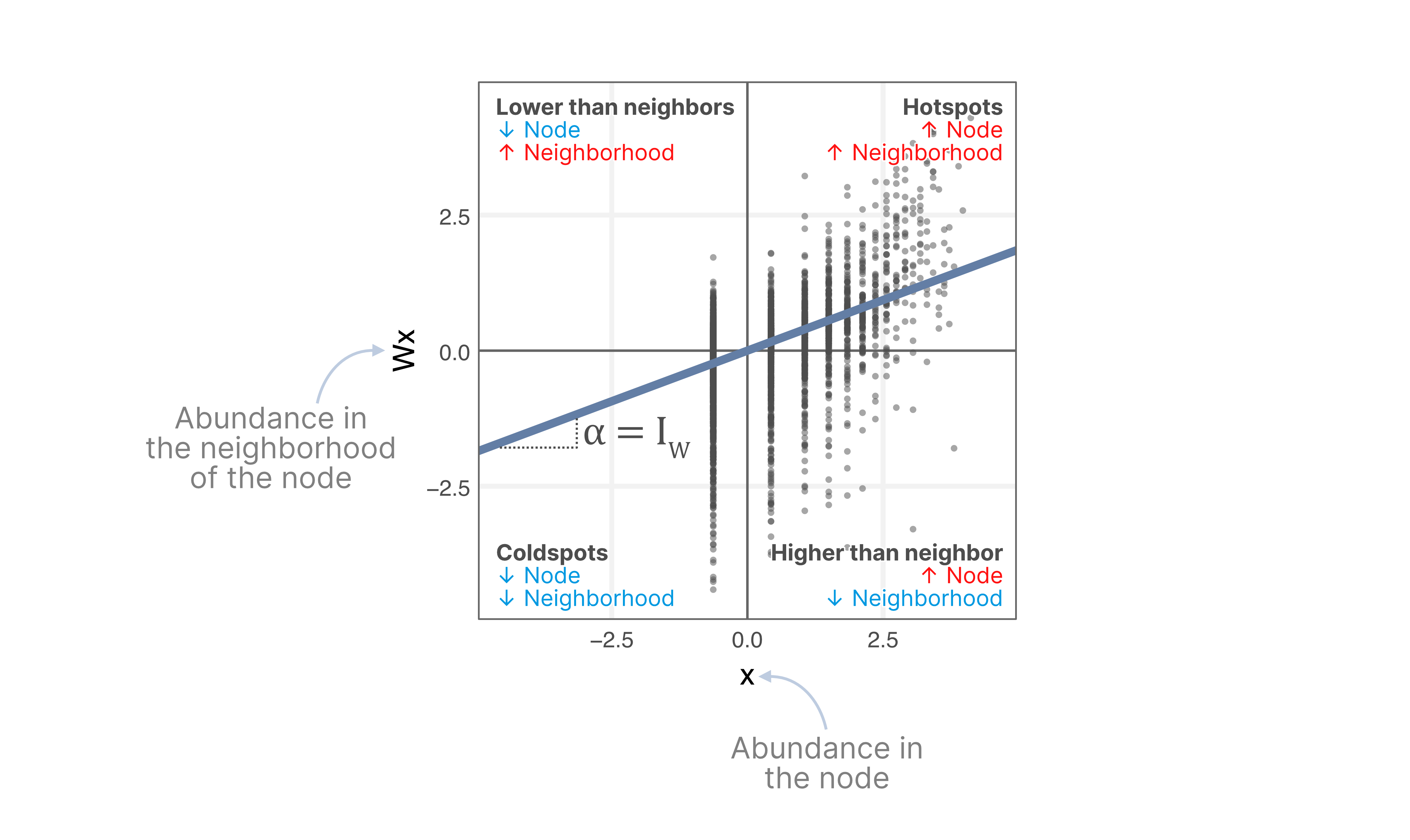
In the context of MPX, Moran’s I measures the global degree of spatial clustering of a protein
within the MPX graph component
(the cell). The value of Moran's I ranges from -1 (perfectly dispersed) to 1 (perfectly clustered),
with 0 representing no
spatial autocorrelation, indicating that the protein is randomly distributed. Moran’s I can be
expressed as a Z-score
(morans_z), which is calculated as the number of standard deviations that the Moran's I statistic
deviates from the
expected mean of a random distribution. Pixelator performs
a Monte Carlo simulation
to estimate the random null distribution, allowing the polarity score to be expressed as
a Z-score.
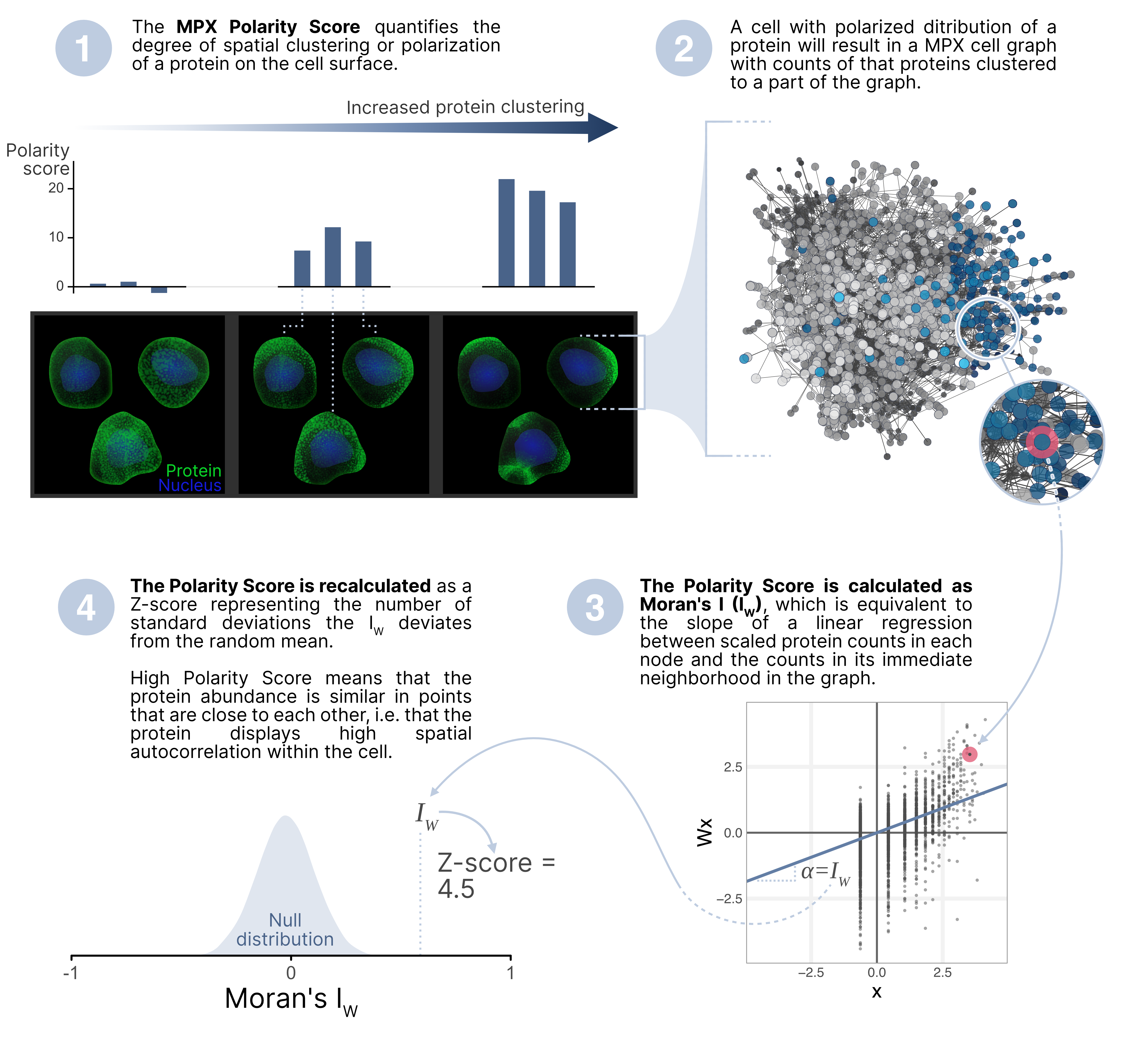
It is important to note that the MPX Polarity Score only measures spatial clustering, which doesn't necessarily mean that only a single pole of protein is present. Instead, a high polarity score could indicate either that the protein has formed a single pole or multiple hotspots of high density of protein molecules on the cell surface.

MPX Colocalization Scores
The MPX colocalization score is a metric to assess how frequently two proteins co-occur within small neighborhoods on the cell surface. High colocalization implies that both proteins are often found in close proximity, while low colocalization indicates they are usually apart.
The metrics used to assess colocalization in MPX is Pearson correlation (pearson), which measures
the linear relationship between the counts of two markers in an A pixel and its immediate
neighboring A pixels. Pixelator also performs a
Monte Carlo simulation to estimate the degree of
colocalization that would
occur by random chance. This allows the actual colocalization score to be expressed as
a Z-score.
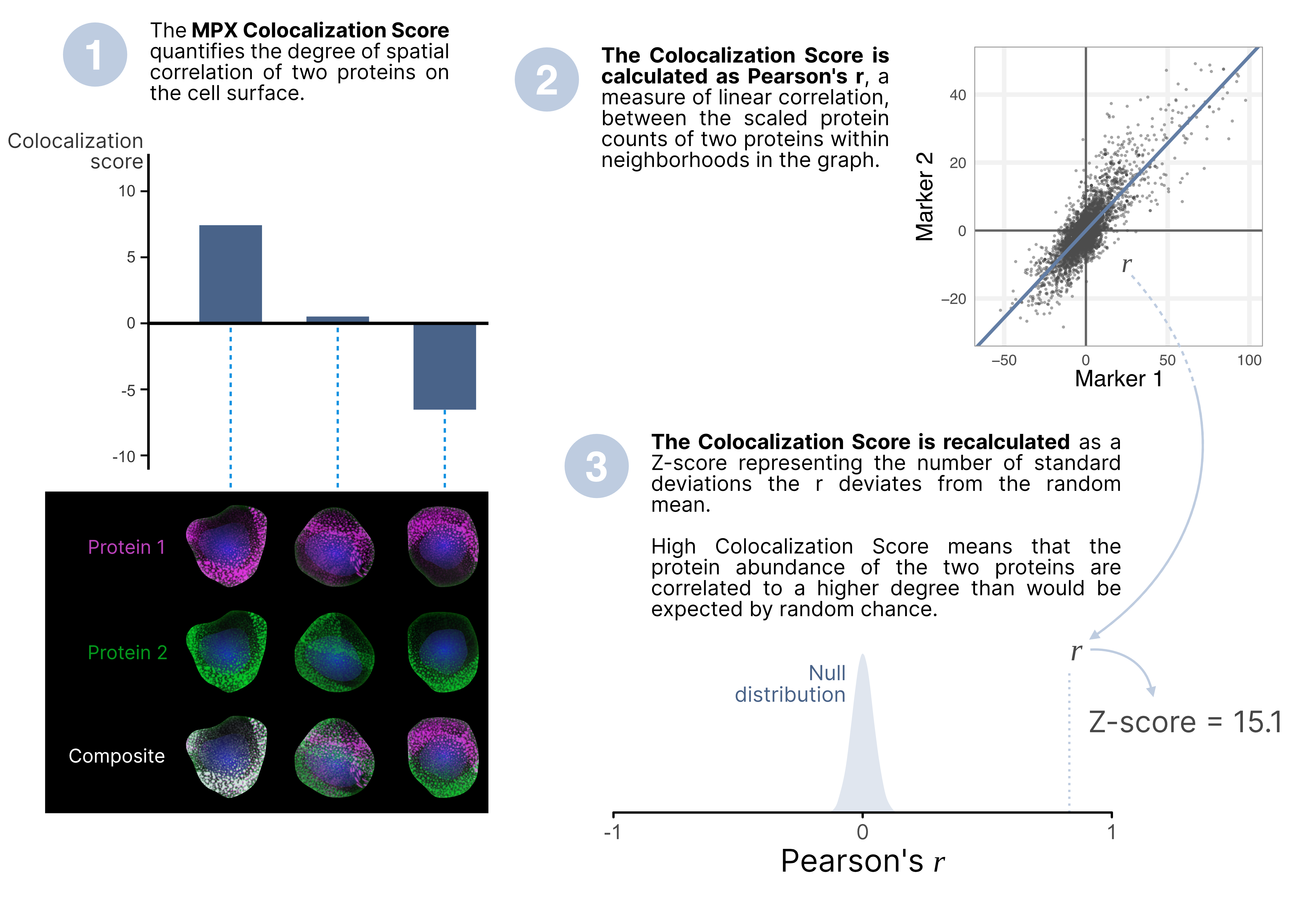
It is important to understand that a high colocalization score does not necessarily mean the proteins form a single complex. Instead, it suggests that they are frequently found in the same regions or hotspots on the cell surface. Negative colocalization score could indicate segregation of two markers, suggesting that the proteins are spatially separated and tend not to be found in the same regions or hotspots on the cell surface.
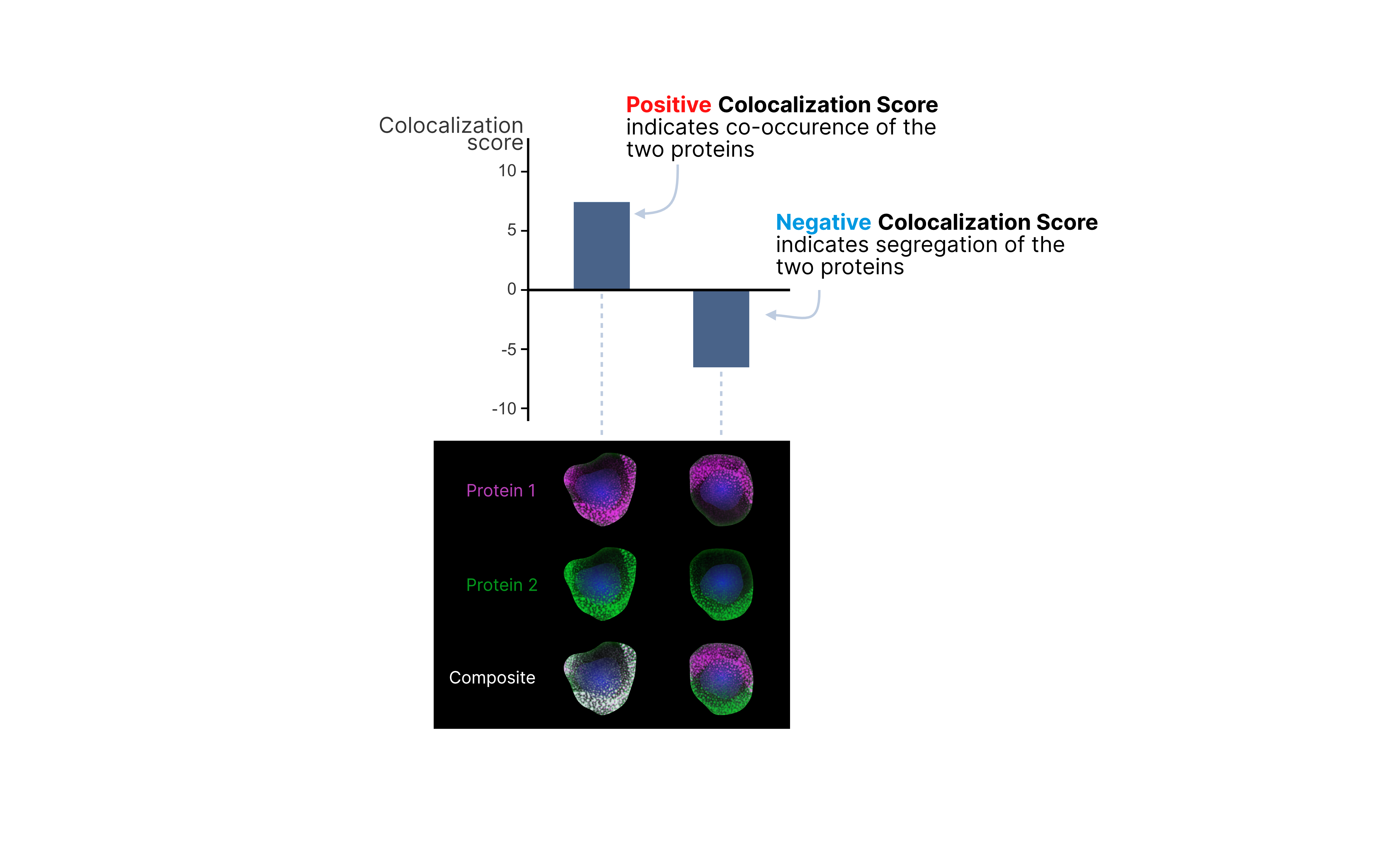
To compute colocalization, we use a transformation of protein counts that we refer to as rate-diff. The rate-diff value of protein in neighborhood is the difference between the raw count of that protein and its expected count in that neighborhood.
The expected count of a protein in a neighborhood is calculated based on the total number of molecules in that neighborhood and the protein's frequency in the component ( cell) .
For example, if of the molecules from a cell correspond to CD45 proteins (i.e. ), in a neighborhood with molecules, we would expect CD45 proteins. If we observe CD45 proteins in that neighborhood, the rate-diff value for CD45 in that neighborhood would be .
Spatial Z-scores
The Z-score of the spatial metrics is a statistical measure used to determine the significance of spatial patterns observed on the cell surface. The Z-scores provide a way to normalize the colocalization and polarity metrics to relate them to the level of spatial structure that is expected by random chance, given a graph's structure and protein levels.
The calculation of Z-scores involves comparing the observed metric (such as Pearson correlation, Jaccard index, or Moran's I) to a distribution of values expected under a null hypothesis of random distribution. This null distribution is in Pixelator generated through Monte Carlo simulation, where the spatial arrangement of proteins in each graph (each corresponding to a cell) is randomized multiple times to create a baseline expectation. This generates a model in which the protein levels remain constant but proteins are distributed randomly across the cell surface, lacking any spatial structure.
A Z-score is then calculated as the number of standard deviations by which the observed metric deviates from the mean expected under the null hypothesis of random distribution:
where is the observed metric, is the mean of the null distribution, and is the standard deviation of the null distribution.
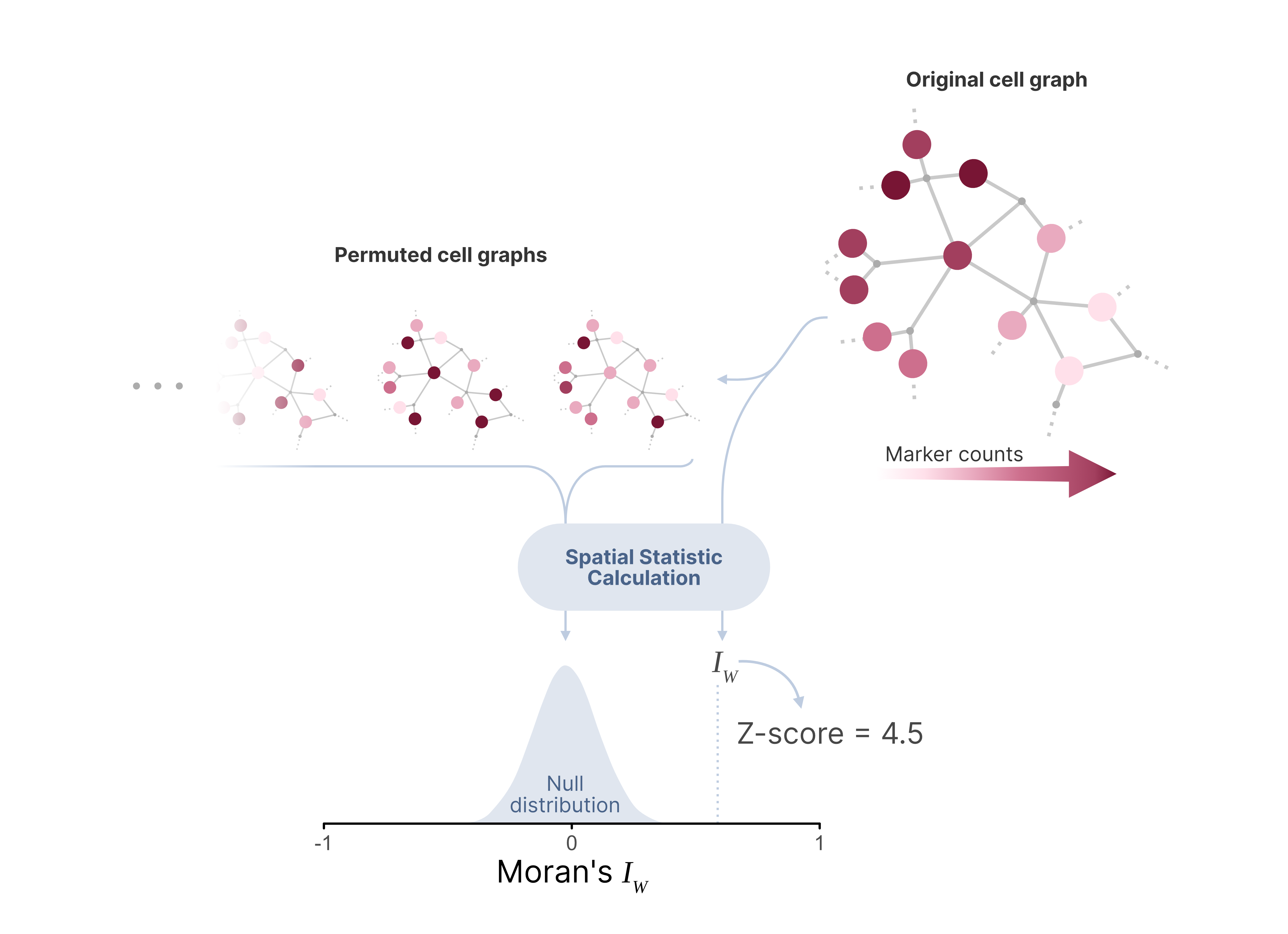
A positive Z-scores indicate that the observed spatial pattern (such as clustering or colocalization) is stronger than expected by chance, while a negative Z-scores suggest weaker patterns than would be expected by random chance. A Z-score close to zero implies that the spatial distribution of proteins does not significantly deviate from randomness.
In the context of MPX, Z-scores are helpful for interpreting the biological significance of protein distribution patterns. They help to distinguish between genuine biological phenomena and random variability, to promote robust and reliable conclusions.
Local
Local ("gi"), also known as Getis-Ord statistic, is a statistic used to find regions of a given study area where some measured variable of interest clusters. A classical application of this statistic is to identify local spatial autocorrelation patterns or "hot spots" where the variable of interest takes higher or lower values than expected. The study area is typically represented as a map, with measurements taken at specific sites. Using information about the relative distances between the sites, we can define local neighborhoods around each site. The local statistic then quantifies the degree to which the variable of interest clusters within these neighborhoods relative to the entire study area.
In MPX data analysis, the study area is a graph and the measured values are protein marker counts. Here, the marker counts are found in the nodes of the graph, and while we do not know the exact spatial positions of the nodes, we can define neighborhoods using the edges of the graph instead. One useful application of local in this context is to identify regions of a cell component graph where a marker of interest has a higher abundance than expected which is the case for polarization events.
Low-abundance markers can be of significant interest but are typically sparsely distributed in a cell component graph, making it challenging to identify and visualize spatial patterns such as polarization events. By summarizing abundance information across neighborhoods, the local statistic reduces the limitations of sparse data and becomes a valuable tool for creating more interpretable 3D visualizations of polarized marker expression.
Definition
Local is a Z-score that quantifies the deviation of the observed local marker expression from the expected expression under the null hypothesis of no spatial clustering. The sign of the score indicates whether the observed marker counts are higher or lower than expected, thus identifying hot and/or cold spots.
The local metric is calculated using the following formula (Ord and Getis, 1995, equation 6):
where
and
In this equation for , the condition that is central. An alternative definition, denoted ("gstari") relaxes this constraint, by including as a neighbor of itself. This statistic is expressed as (Ord and Getis, 1995, equation 7):
where
and
Both methods ("gi" and "gstari") are implemented in the pixelator (Python) and pixelatorR (R) analysis tool kits.
If we apply local or local on cell component data, corresponds to node counts for a selected protein marker. The statistic is calculated for a single node , using information about protein marker abundance () in the local neighborhood of . This neighborhood could for example consist of the direct neighbors to in the graph. We can also expand the neighborhood around to include nodes that are up to steps away. The effect of increasing the neighborhood size is that the spatial scale is increased, and we can identify larger spatial patterns in the graph. For visualization purposes, increasing can be an effective strategy to highlight large spatial patterns such as polarization events.
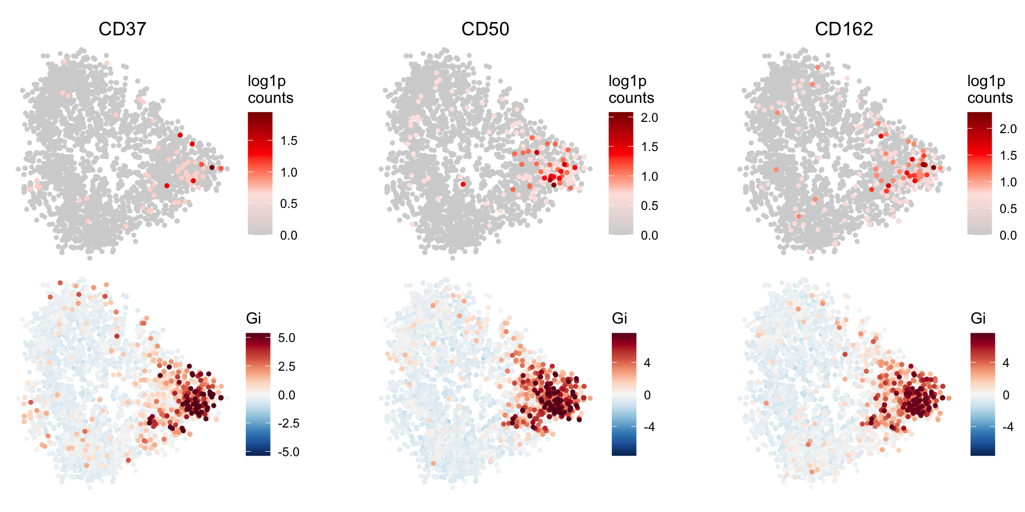 Local G scores reveal a polarization pattern in a cell component graph. The figure displays data
for three protein markers: CD37, CD50, and CD162. The top row presents the log1p-transformed counts
for each marker, while the bottom row illustrates the corresponding local G scores. Each point
corresponds to a node in the graph.
Weights in Local
The marker counts in nodes of a component graph are correlated with the degree of the nodes. If this is not accounted for, high degree nodes will contribute more to the statistic. Additionally, if we set to a value larger than 1 to include neighbors that are more than 1 step away from , we need to assign lower weights to nodes that are further away. For these reasons, the Local G algorithm that we provide in pixelator (Python) and pixelatorR (R) also computes edge weights between and its neighbors (). These edge weights are based on transition probabilities between nodes, and aim to correct for the degree bias and the distance between nodes within the neighborhood.
MPX layouts
Cell component graphs can be visualized in 3D layouts using graph drawing techniques. These often aim to create layouts that are visually intuitive, making it easier to identify and interpret group structures and relationships among nodes, highlighting key features such as clusters, hierarchies, and pathways within the data. For instance, in social network analysis, it is common to draw a 2D layout of the network that highlights community structure. However, MPX graphs are distinct from many other types of graphs because they contain information about spatial relationships. Here, the goal is to find a 3D layout of the graph that gives an abstract representation of the structure of the cell.
Pixelator offers options to compute layouts for each MPX component in a data set using three different algorithms: Fruchterman-Reingold (FR), Kamada-Kawai (KK), and pivot Multidimensional Scaling (pMDS). The FR and KK algorithms are force-directed methods that assign forces to edges and nodes, and then allow these forces to repel and attract each other until the nodes reach a mechanical equilibrium. A major limitation with force-directed algorithms is the high running time, which in general is considered to run in cubic time O(N^3). This limitation presents a computational challenge as an MPX data set consists of hundreds to thousands of relatively large graphs. For additional details on these methods, please refer to the following articles:
The pMDS technique, which is the default graph drawing method in Pixelator, overcomes the running time limitations with force-directed algorithms. It builds on the same principles as classical multidimensional scaling ( MDS), a widely studied method for graph drawing that converts distances between pairs of nodes into a configuration of points in an abstract Euclidean space. In brief, given the shortest path distances between each pair of nodes in the graph, the MDS technique attempts to place each node in a low-dimensional space (typically 2D or 3D) such that the distances between nodes in this space reflect the original distances as closely as possible. If we consider an MPX graph, we know that nodes that are connected by an edge should in theory correspond to DNA pixels that are positioned close to each other on the cell surface. Knowing that edges correspond to proximity relationships make MDS a good candidate for graph drawing of MPX component graphs.
While classical MDS also suffers from a high running time, this is mitigated with pMDS (Brandes et al.). Instead of computing all pairwise distances, pMDS only considers the shortest path distances from all nodes to a set of randomly selected "pivot" nodes. Below, we outline the general steps of the algorithm for computing a 3D graph layout:
Pivot MDS Input: an undirected graph , pivot nodes where
Steps:
- Select random pivot nodes from
- Compute the shortest path distances for nodes to pivot nodes to yield a distance matrix . For unweighted graphs, we can use a Breadth-First Search (BFS) to compute the distances.
- Create a transformed distance matrix , which is double-centered
- Decompose with Single Value Decomposition (SVD) and select the three singular vectors with the highest singular values
- The layout coordinates are obtained by computing:
Weighted pMDS
In the PMDS algorithm described earlier, the shortest path distances are computed for an unweighted graph, meaning all edges are considered to have equal weight. However, in the context of MPX data, the physical distance between pixels varies, and treating all edges the same does not accurately represent this variability. To improve the Pivot MDS layouts, edges can be weighted when computing the shortest path distances.
In Pixelator, we provide a method to calculate edge weights based on transition probabilities within the graph. The underlying assumption is that the transition probability between two nodes reflects the physical distance between their corresponding pixels. A low transition probability implies that the pixels are far apart, while a high transition probability suggests that the pixels are close to each other.
When using weighted pMDS in Pixelator, edge weights are automatically calculated based on transition probabilities. Dijkstra's algorithm is then used to compute the shortest path distances (step 2 in the pMDS algorithm) which is the appropriate choice for weighted graphs. These weighted shortest path distances are subsequently used to determine the layout coordinates in the same manner as the unweighted pMDS algorithm. This weighting scheme results in layouts that more accurately reflect the physical distances between pixels on the cell surface, leading to more precise and interpretable layouts.