Multiple Comparisons of Abundance and Spatial Scores

In many biological analyses, researchers focus on comparing a single condition or cell type to a specific reference group. For example, they might compare B cells to CD4 T cells or examine treated versus control monocytes. However, there are scenarios where investigating and comparing multiple experimental conditions, cell types, or time points against a single reference group can yield valuable insights. Traditionally, one approach to achieve this has been to manually loop over samples or conditions in the metadata slot of a PXL file object, running multiple tests in succession. While effective, this method can be time-consuming and prone to error.

As we will demonstrate in this tutorial, differential abundance testing using the rank_genes_groups function from Scanpy has this functionality out of the box. Recent extensions to the pixelator functions get_differential_polarity and get_differential_colocalization now offer a more streamlined approach to do the same for the spatial score testing. These updated functions allow for multi-group comparisons without the need to set up complex looping code.

By the end of this tutorial, you will be able to:

• Perform differential abundance, polarization, and colocalization tests comparing multiple groups to a single reference group.
• Utilize the enhanced capabilities of get_differential_polarity and get_differential_colocalization for efficient multi-group analyses.
• Visualize the results from these complex comparisons using plot_polarity_diff_volcano and plot_colocalization_diff_volcano.

Setup

import numpy as np
import pandas as pd
from pathlib import Path
from pixelator.mpx import read, simple_aggregate
from pixelator.common.statistics import dsb_normalize
from pixelator.mpx.analysis.polarization import get_differential_polarity
from pixelator.mpx.analysis.colocalization import get_differential_colocalization
from pixelator.mpx.plot import plot_colocalization_diff_volcano, plot_polarity_diff_volcano
import seaborn as sns
import scanpy as sc
import matplotlib.pyplot as plt
from scipy.stats import mannwhitneyu, false_discovery_control, zscore
from statsmodels.stats.multitest import multipletests
import umap

sns.set_style("whitegrid")

Loading data

To demonstrate the multiple comparison functionality, we’ll revisit the uropod data first introduced in the spatial analysis tutorial. As a refresher, this experiment involves T cells immobilized with CD54 and stimulated with either RANTES or MCP1 to induce uropod formation. A uropod is a protrusion on the cell surface that aids in cellular movement. During uropod formation, certain surface proteins migrate to one pole of the cell, creating a bulge. This process can be captured by MPX and is evident in the data as increased polarization and colocalization of the proteins involved in uropod formation. To start off this tutorial, we’ll begin by downloading and loading the required PXL files.

DATA_DIR = Path("<path to the directory to save datasets to>")

And then proceed in Python.

# The folders the data is located in:
data_files = [
    DATA_DIR / "Uropod_CD54_fixed.layout.dataset.pxl",
    DATA_DIR / "Uropod_CD54_fixed_RANTES_stimulated.layout.dataset.pxl",
    DATA_DIR / "Uropod_CD54_fixed_MCP1_stimulated.layout.dataset.pxl",
] 

datasets = list([read(path) for path in data_files])
obj = simple_aggregate(
      ["Control", "Rantes", "Mcpi"], datasets
  )
obj

Pixel dataset contains:
  AnnData with 1607 obs and 80 vars
  Edge list with 20651890 edges
  Polarization scores with 80583 elements
  Colocalization scores with 2160250 elements
  Contains precomputed layouts
  Metadata:
    samples: {'Control': {'version': '0.19.0', 'sample': 'Uropod_CD54_fixed', 'analysis': {'params': {'polarization': {'polarization': {'transformation': 'log1p', 'permutations': 50, 'min_marker_count': 5, 'random_seed': None}}, 'colocalization': {'colocalization': {'transformation_type': 'rate-diff', 'neighbourhood_size': 1, 'n_permutations': 50, 'min_region_count': 5, 'min_marker_count': 5}}}}}, 'Rantes': {'version': '0.19.0', 'sample': 'Uropod_CD54_fixed_RANTES_stimulated', 'analysis': {'params': {'polarization': {'polarization': {'transformation': 'log1p', 'permutations': 50, 'min_marker_count': 5, 'random_seed': None}}, 'colocalization': {'colocalization': {'transformation_type': 'rate-diff', 'neighbourhood_size': 1, 'n_permutations': 50, 'min_region_count': 5, 'min_marker_count': 5}}}}}, 'Mcpi': {'version': '0.19.0', 'sample': 'Uropod_CD54_fixed_MCP1_stimulated', 'analysis': {'params': {'polarization': {'polarization': {'transformation': 'log1p', 'permutations': 50, 'min_marker_count': 5, 'random_seed': None}}, 'colocalization': {'colocalization': {'transformation_type': 'rate-diff', 'neighbourhood_size': 1, 'n_permutations': 50, 'min_region_count': 5, 'min_marker_count': 5}}}}}}

Since quality control and filtering are not the primary focus of this tutorial, we will only perform minimal steps in these areas. However, it’s important to note that thorough quality control and appropriate filtering are crucial for ensuring the reliability and accuracy of your analysis results. For this demonstration, we’ll implement basic quality control measures and apply some essential filtering criteria to prepare our data for further analysis.

QC & Filter Data

edge_rank_df = obj.adata.obs[["sample", "molecules"]].copy()
edge_rank_df["rank"] = edge_rank_df.groupby(["sample"])["molecules"].rank(
    ascending=False, method="first"
)
edgerank_plot = (
    sns.relplot(data=edge_rank_df, x="rank", y="molecules", hue="sample", aspect=1.6)
    .set(xscale="log", yscale="log")
    .set_xlabels("Component rank (by number of molecules)")
    .set_ylabels("Number of molecules")
)
edgerank_plot

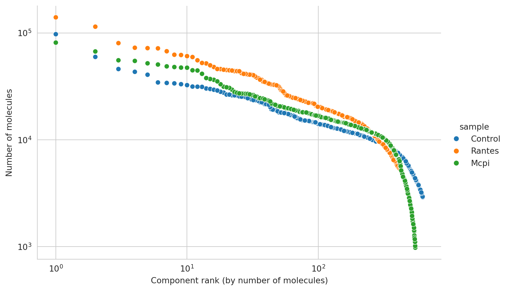
Prior to downstream analysis, we will remove components with less than 3000 molecules as well as the antibody count outliers.

# Add rank to the object for further filtering
obj.adata.obs = obj.adata.obs.join(edge_rank_df["rank"], how="left")

# Remove components with less than 3000 molecules
obj.adata = obj.adata[obj.adata.obs["molecules"] > 3000]
# Only keep the components where tau_type is normal
obj.adata = obj.adata[obj.adata.obs["tau_type"] == "normal"]

Differential Abundance

Prior to running the differential abundance test, we normalize the data.

# Add dsb values as a layer to the object
obj.adata.layers["dsb"] = dsb_normalize(
    obj.adata.to_df(), 
    isotype_controls = ["mIgG1", "mIgG2a", "mIgG2b"]
    )

# Calculate minimum value per marker - See the Normalization tutorial for more details
mins = obj.adata.to_df("dsb").min()
# If minimum value is positive, set to zero
mins[mins > 0] = 0
# Add layer to use in Differential Abundance test
obj.adata.layers["shifted_dsb"] = obj.adata.to_df("dsb").sub(mins)

To perform differential abundance testing across multiple conditions, we use the rank_genes_groups function from Scanpy.

The end result is a dataframe containing differential abundance results for all conditions, with adjusted p-values to account for multiple comparisons. This approach streamlines the analysis process and facilitates easier interpretation of results across different experimental conditions.

targets = ["Rantes", "Mcpi"]
reference = "Control"

# Run a wilcoxon test to compare groups
sc.tl.rank_genes_groups(
    obj.adata,
    groupby="sample",
    method="wilcoxon",
    layer="shifted_dsb",
    groups=targets,
    reference="Control",
    correction_method="BH"
)

# Collect results and calculate -log10(adjusted p-value) for plotting
diff_exp_df = sc.get.rank_genes_groups_df(obj.adata, group=None)
diff_exp_df["-log10(adjusted p-value)"] = -np.log10(diff_exp_df["pvals_adj"])
diff_exp_df["label"] = (diff_exp_df["pvals_adj"] < 0.01) & (abs(diff_exp_df["logfoldchanges"]) > 0.5)  

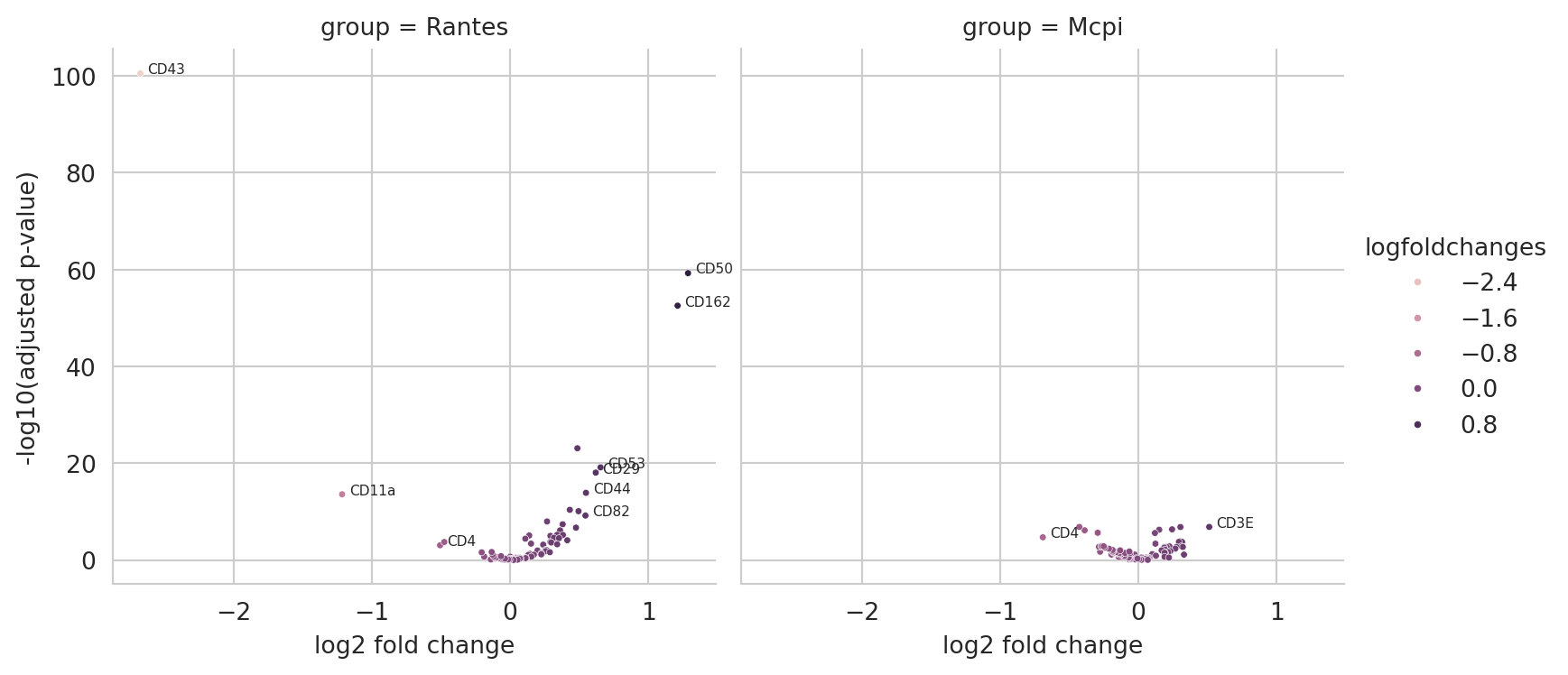
We can visualize the results of this differential analysis as a volcano plot using functions presented in the Abundance Normalization tutorial.

diff_abund_plot = (
    sns.relplot(
    diff_exp_df,
    x="logfoldchanges",
    y="-log10(adjusted p-value)",
    hue="logfoldchanges",
    col="group",
    col_wrap=2,
    height=4,
    s=8,
).set_xlabels("log2 fold change")
)

for text, row in diff_exp_df[diff_exp_df["label"]].iterrows():
    x, y, group = row[["logfoldchanges", "-log10(adjusted p-value)", "group"]]
    if group == diff_exp_df["group"].unique()[0]:
        which_axis = 0
    else:
        which_axis = 1 
    label = diff_abund_plot.axes[which_axis].text(
        x + 0.05, y, diff_exp_df.loc[text, "names"] , horizontalalignment="left", fontsize="xx-small"
    )

diff_abund_plot

Differential Polarization

In this section, we’ll explore how to perform differential polarization testing, comparing both RANTES and MCP1 treatments against a control reference. While typical workflows often begin with filtering steps to remove lowly abundant markers, we’ll omit that for this demonstration.

We’ll highlight a new feature of the get_differential_polarity function from the pixelator package. As mentioned before, comparing multiple conditions to a single reference group used to require iterative approaches and/or data subsetting. However, the updated get_differential_polarity function streamlines this process. It accepts multiple experimental conditions to be tested against a single reference group in one operation. This functionality not only saves time but also automatically handles p-value adjustments for multiple comparisons (Bonferroni correction by default). By leveraging this feature, we can simultaneously assess the differential polarization effects of both RANTES and MCP1 treatments compared to the control condition.

targets = ["Rantes", "Mcpi"]
reference = "Control"

DPA = get_differential_polarity(obj.polarization,
    targets = targets,
    reference = "Control",
    contrast_column = "sample")

DPA.sort_values(by =['p_adj'])

	marker	stat	p_value	median_difference	p_adj	target
15	CD162	57482.0	6.490396e-46	3.276248	5.192317e-44	Rantes
57	CD50	69329.0	6.749971e-24	2.484719	5.399977e-22	Rantes
28	CD26	97543.0	2.133449e-12	1.042112	1.706759e-10	Rantes
70	CD82	101036.0	5.078217e-11	0.788962	4.062574e-09	Rantes
17	CD18	104385.0	1.747884e-10	0.908812	1.398307e-08	Rantes
...	...	...	...	...	...	...
75	HLA-DR	177188.0	1.143129e-01	-0.146772	1.000000e+00	Mcpi
76	TCRVb5	81015.0	5.179407e-01	0.041924	1.000000e+00	Mcpi
77	mIgG1	17007.0	7.778279e-01	-0.028209	1.000000e+00	Mcpi
78	mIgG2a	38053.0	1.518312e-01	-0.123990	1.000000e+00	Mcpi
79	mIgG2b	48753.0	3.982969e-01	0.056669	1.000000e+00	Mcpi

160 rows × 6 columns

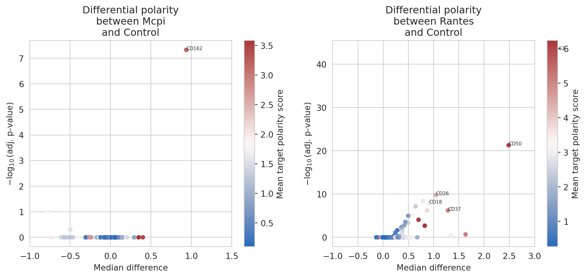
Alternatively, we can visualize the output of these tests next to each other in a facetted volcano plot. The plot_polarity_diff_volcano function will perform the differential analysis and create volcano plots facetted on the targets.

# Create polarity strip plot

pol_volcano_plot = plot_polarity_diff_volcano(obj.polarization,
    targets = targets,
    reference = "Control",
    contrast_column = "sample")
_ = pol_volcano_plot[1][0].set_xlim(-1, 1.5)
_ = pol_volcano_plot[1][1].set_xlim(-1, 3)

Differential Colocalization

Similarly, we can run multiple differential colocalization tests from a single call to get_differential_colocalization.

DCA = get_differential_colocalization(obj.colocalization,
    targets = targets,
    reference = "Control",
    contrast_column = "sample")

DCA.sort_values(by =['p_adj'])

	marker_1	marker_2	stat	p_value	median_difference	p_adj	target
1121	CD162	CD50	60522.0	1.990746e-28	7.118788	6.290758e-25	Rantes
151	B2M	HLA-ABC	90377.0	2.380435e-20	4.897676	7.522174e-17	Rantes
1241	CD18	CD45RB	93332.0	1.790114e-17	3.771053	5.656759e-14	Rantes
2138	CD29	CD43	101524.0	8.688518e-16	-3.437684	2.745572e-12	Rantes
1114	CD162	CD45	157426.0	1.085987e-15	-3.713952	3.431718e-12	Rantes
...	...	...	...	...	...	...	...
3156	TCRVb5	mIgG2b	39590.0	2.514257e-01	-0.386695	1.000000e+00	Mcpi
3157	mIgG1	mIgG2a	10733.0	1.917360e-01	-0.804866	1.000000e+00	Mcpi
3158	mIgG1	mIgG2b	11533.0	6.731368e-01	-0.226777	1.000000e+00	Mcpi
3159	mIgG2a	mIgG2b	19345.0	7.051521e-01	0.176204	1.000000e+00	Mcpi
0	ACTB	B2M	14082.0	9.354814e-01	0.079239	1.000000e+00	Rantes

6320 rows × 7 columns

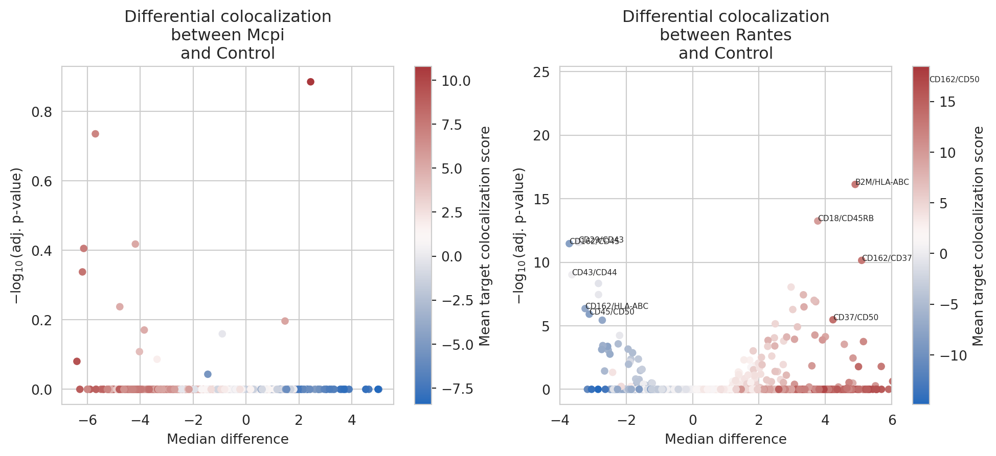
Again, side-by-side visualization of the volcano plots is easily achieved by facetting on the targets using the plot_colocalization_diff_volcano function. This function will perform the differential analysis and create volcano plots facetted on the targets.

# Volcano plot
col_volcano_plot = plot_colocalization_diff_volcano(obj.colocalization,
    targets = targets,
    reference = "Control",
    contrast_column = "sample")

_ = col_volcano_plot[1][1].set_xlim(-4, 6)

This concludes this short tutorial on performing multiple comparisons of abundance, polarization, and colocalization. Now, you’ll be able to perform multiple comparisons simultaneously, which significantly accelerates the analysis process for more complex experimental designs. The combination of speed, accuracy, and statistical robustness provided by this approach will help ensure that your results are not only more reliable but also more likely to stand up to peer review and replication efforts.

Remember, while this method is powerful, it’s always important to consider the biological context of your experiments and interpret the results in light of your specific research questions and hypotheses.